Update (July 2026): The model has since been substantially reworked around an equipercentile backbone, with much better accuracy. The original post below describes the first version; see the update at the end for what changed.
Every year, thousands of Bulgarian 7th graders face a stressful decision: which high schools to apply to based on their NVO (Национално външно оценяване) exam scores. The challenge? Admission cutoffs vary wildly year-to-year, making it hard to know if you’ll get in.
I built an ML system to predict these cutoffs and help families make informed decisions.
Why I Built This
My stepdaughter is taking the NVO this year. As we started researching schools, I realized how frustrating the process is - you’re essentially guessing which schools she might qualify for based on outdated data.
Looking at last year’s cutoffs is misleading. One school we liked had a cutoff of 455 in 2024, but jumped to 478 in 2025. Another dropped from 470 to 441. Without understanding these patterns, families are essentially gambling with their applications.
I thought: there’s historical data available, patterns exist - why not try to predict this? At minimum, it would help us make better decisions. At best, it might help other families too.
The Problem
Predicting admission scores is genuinely hard:
- Exam difficulty changes yearly - An “easy” math exam means higher scores across the board
- Student preferences shift - A school gains or loses popularity
- Capacity changes - New programs open, others close
- Competition fluctuates - Demographics and student counts vary
The naive approach (just use last year’s score) works surprisingly well for stable schools, but fails badly for volatile ones. Some schools swing 50-100 points between years.
The Key Insight: Predict the Delta
Instead of predicting absolute scores (e.g., “this school will have a 465 cutoff”), I predict the year-over-year change.
Why? Because last year’s score is by far the strongest predictor. The model’s job is to learn: “given this school’s history and this year’s exam distribution, will the cutoff go up or down, and by how much?”
This reframing made the problem tractable. The model predicts deltas like +12 or -8, then adds them to the previous year’s score.
Feature Engineering
The features that matter most:
| Feature | Why It Helps |
|---|---|
| Previous year score | Strongest predictor - schools tend to stay in their “tier” |
| Historical volatility | High-variance schools are harder to predict |
| Trend direction | Is this school trending up or down over 3+ years? |
| Distance from mean | Schools far from their historical average tend to regress |
| Exam percentiles | Harder exams shift all cutoffs down |
I also discovered that acceleration matters - if a school jumped +30 last year after +20 the year before, it might be on a trajectory.
The Model
I used XGBoost with deliberately shallow trees (max_depth=3) and strong regularization. With only ~800 training samples (3 years × ~270 schools), overfitting is the main enemy.
model = xgb.XGBRegressor(
    n_estimators=50,
    max_depth=3,
    learning_rate=0.1,
    reg_alpha=1.0,
    reg_lambda=2.0
)
Training takes under 2 seconds. The simplicity is a feature, not a bug.
A Surprising Discovery: Gender Matters
One unexpected finding: the model helps significantly for female predictions but barely beats the naive baseline for male predictions.
After investigation, I found that female cutoffs are generally more predictable - they have lower volatility and clearer trends. Male cutoffs have more noise.
The solution: gender-specific blending weights.
- Female: 60% model, 40% naive baseline
- Male: 0% model, 100% naive baseline (just use last year’s score)
Sometimes the best model is knowing when not to use a model.
Results
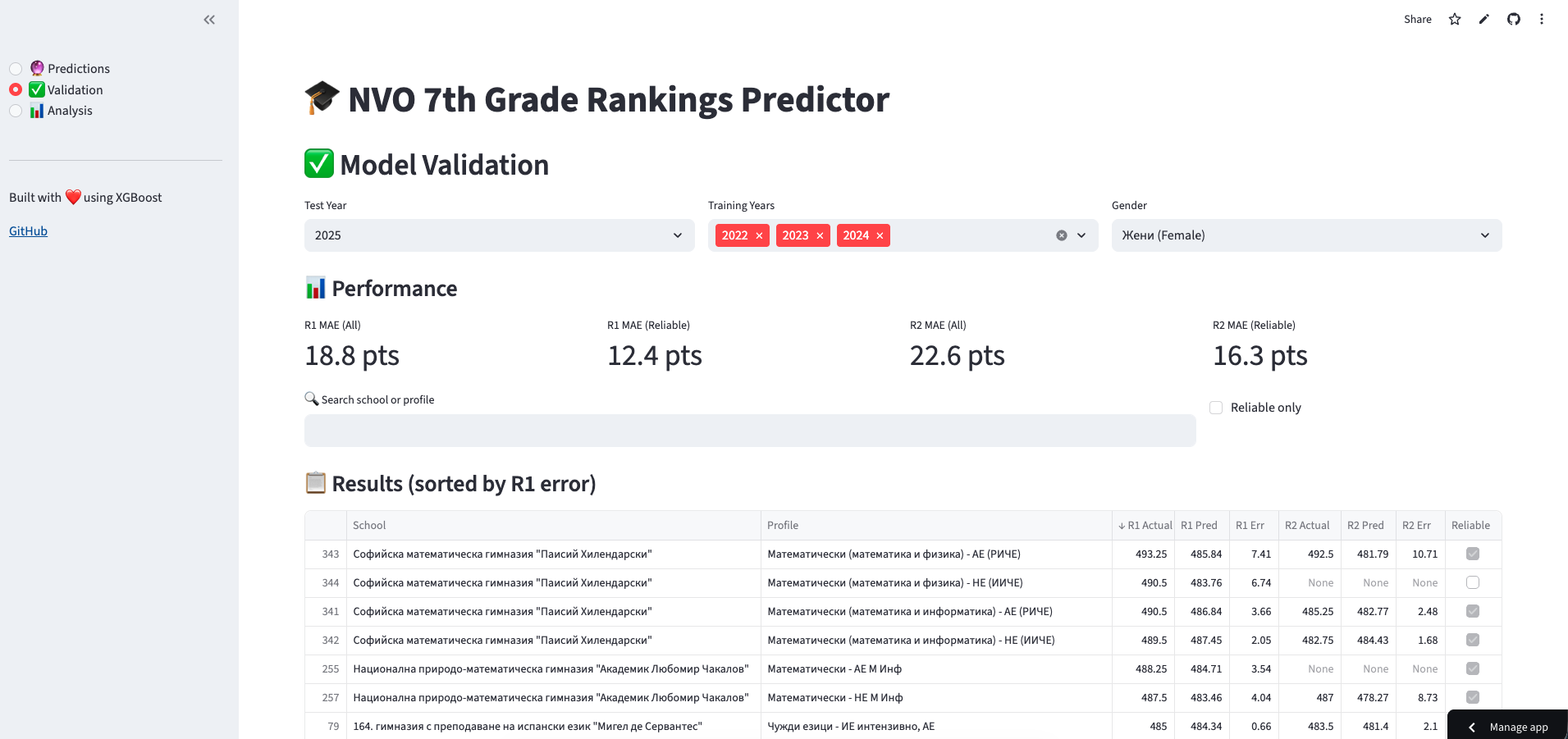
Validated on 2025 data (trained on 2022-2024):
| Metric | All Schools | Reliable Only |
|---|---|---|
| R1 MAE | 19.15 pts | 13.42 pts |
| Within 10 pts | 45.6% | 54.8% |
| Within 20 pts | 65.8% | 77.4% |
“Reliable” predictions = schools with ≥2 years history, volatility <25, and previous year data.
Concrete Example
For the 2025 validation, here’s how predictions compared to reality for some well-known schools:
| School | Profile | Predicted | Actual | Error |
|---|---|---|---|---|
| СМГ | Математика | 487.2 | 489.5 | -2.3 |
| НПМГ | Информатика | 478.5 | 481.0 | -2.5 |
| 91 НЕГ | Английски | 462.1 | 458.3 | +3.8 |
| ТУЕС | Системно програмиране | 455.8 | 461.2 | -5.4 |
For stable, popular schools, predictions are quite accurate. The errors grow for less popular or more volatile programs.
Confidence Intervals
Raw predictions aren’t enough. A prediction of “465” means nothing without context. Is that ±5 points or ±30?
I compute confidence intervals based on each school’s historical volatility:
- Stable school (volatility=8): 465 ± 12 points
- Volatile school (volatility=35): 465 ± 52 points
The UI clearly marks predictions as “Reliable” or not, so users know when to trust them.
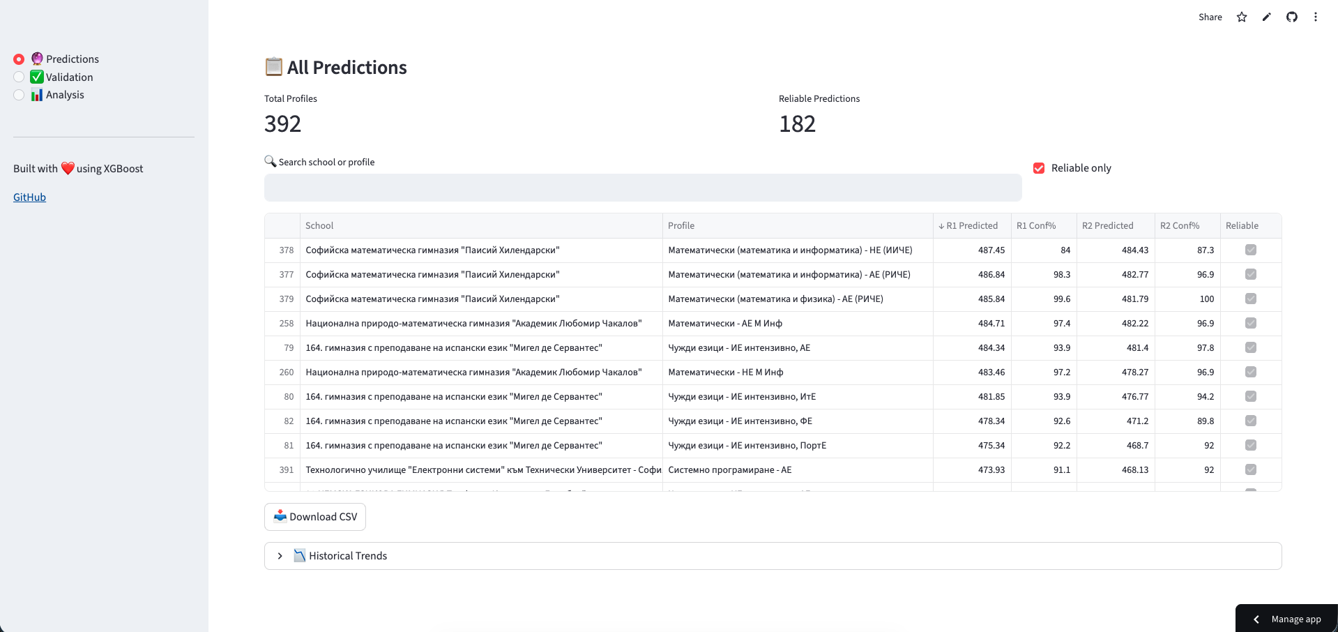
The Web Interface
I built a Streamlit app with three main features:
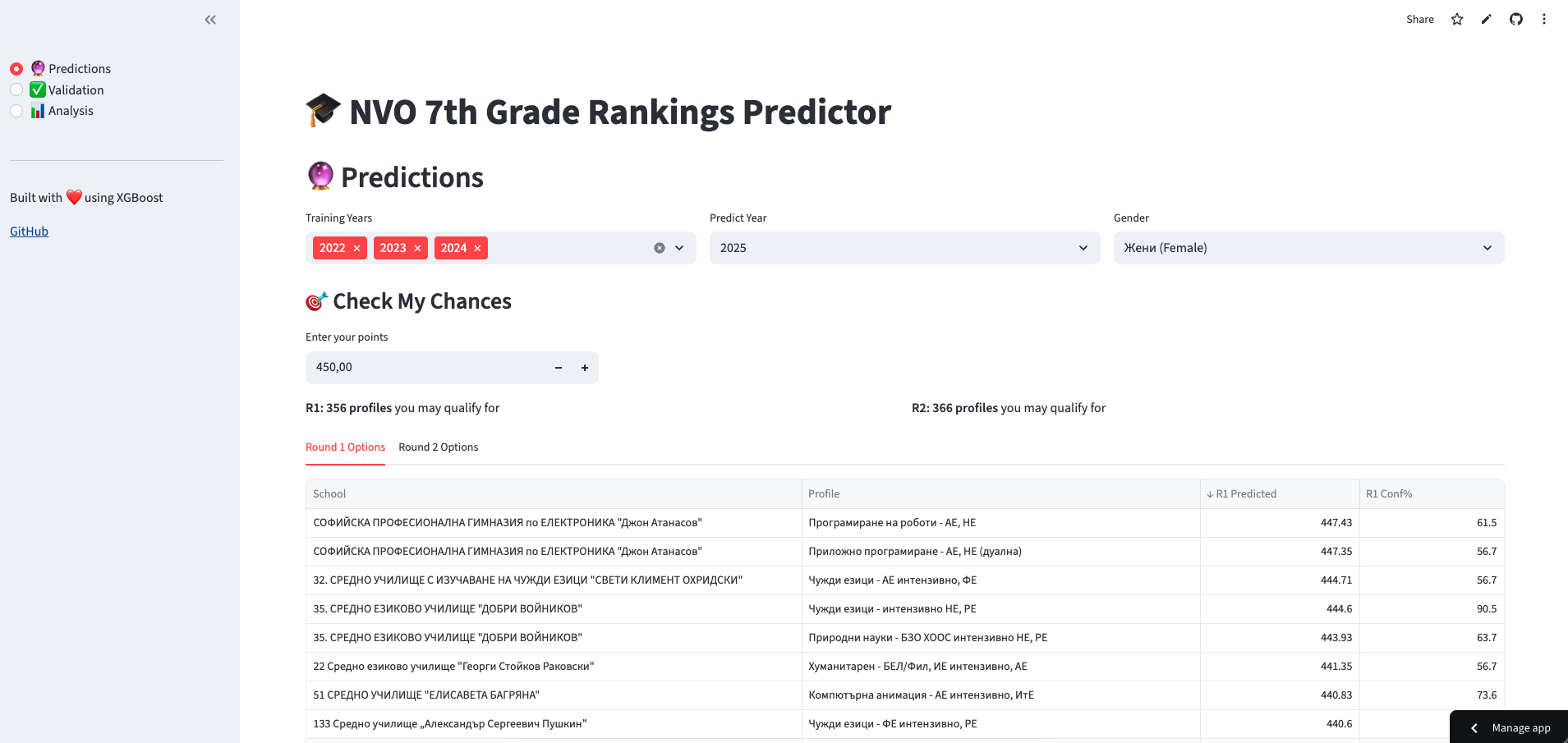
1. Check My Chances - Enter your score, see which schools you might qualify for:
2. Validation View - See how predictions compare to actual results:
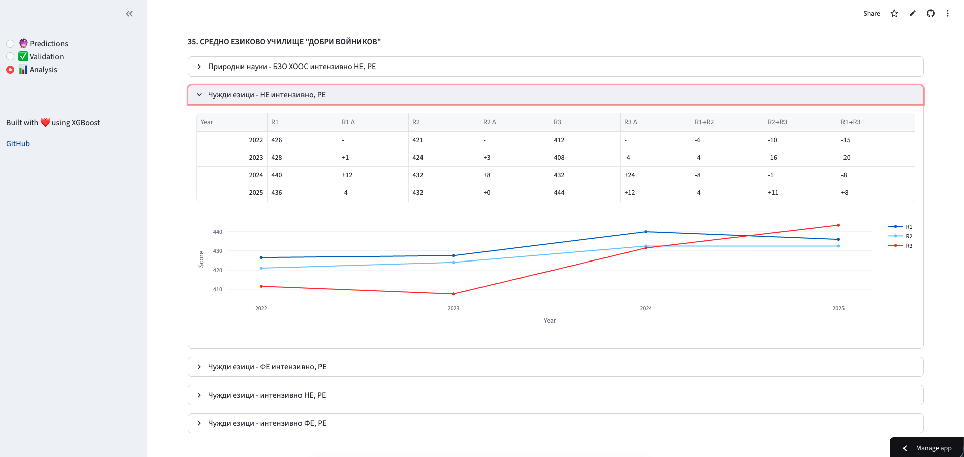
3. Historical Analysis - Explore trends for specific schools:
What I Learned
1. Simple baselines are powerful. Before building anything complex, I checked: what if we just use last year’s score? That baseline was hard to beat, and for male predictions, I couldn’t beat it at all.
2. Confidence matters as much as accuracy. Users don’t just need a number - they need to know how much to trust it. Flagging unreliable predictions prevents false confidence.
3. Domain knowledge beats algorithms. Understanding that schools “regress to mean” and that exam difficulty shifts all scores together - these insights helped more than hyperparameter tuning.
4. Know when to give up. For highly volatile schools (100+ point swings), no model will help. Being honest about limitations builds trust.
Limitations
- Sofia only - Trained on РУО София-град data. Other cities have different dynamics.
- Cold start problem - Can’t predict new schools with no history.
- External shocks - Policy changes, new programs, or demographic shifts aren’t captured.
- Not financial advice - Wait, wrong domain. But seriously: use this as one input, not the only input.
Try It Yourself
The project includes both CLI and web interface:
# Clone and install
git clone https://github.com/zhivko-georgiev/nvo7-predictor.git
cd nvo7-predictor
pip install -e .

# Predict 2026 cutoffs
nvo predict --year 2026 --gender female

# Launch web UI
streamlit run app.py
Check out the code on GitHub, or try the live demo.
What’s Next
Ideas for future improvements:
- Support for other Bulgarian cities
- Better handling of new schools (transfer learning from similar profiles?)
If you’re a parent going through this process, I hope this helps reduce some stress. And if you’re a data scientist - the dataset is interesting and the problem is real. PRs welcome!
Update (July 2026): The Equipercentile Rewrite
The 2026 NVO exams are done, the score distributions are published, and the system is now producing its first real predictions - for the year my stepdaughter actually applies. Before that, the model went through its biggest overhaul yet. Here’s what changed.
The new backbone: equipercentile rank mapping
The original model treated exam difficulty as just another feature and hoped XGBoost would figure it out. That was always the weakest link - tree models can’t extrapolate, so a year with an unusually hard or easy exam would break the predictions.
The fix came from a change in perspective: a school’s prestige is more stable than its cutoff score. СМГ doesn’t get 20 points “worse” because the math exam was harder - it still attracts the same top slice of students. What moves is the score scale underneath.
So instead of predicting scores directly, the model now:
- Converts last year’s cutoff to a percentile rank in last year’s exam score distribution
- Maps that same rank through this year’s distribution
- Converts back to a cutoff score
If a school’s cutoff sat at the 95th percentile last year, it probably sits near the 95th percentile this year too - whatever score that happens to correspond to. Exam difficulty shifts are handled by construction, not learned from data.
ML demoted to residual correction
XGBoost didn’t go away, but it changed jobs. The equipercentile mapping is the base prediction; the model now only predicts the residual - the part of the change not explained by exam difficulty, like trends, mean reversion, and capacity effects. The final prediction blends the two, with the blend weight tuned by leave-one-year-out cross-validation (capped at 0.8 to avoid overfitting to any single year’s regime).
Revisiting “gender matters”
Remember the surprising finding that male predictions were better off ignoring the model entirely (0% model weight)? It turns out much of that “noise” in male cutoffs was exam difficulty variance that the old model couldn’t capture. With the equipercentile backbone absorbing difficulty shifts, the model helps for both genders now, and the blend weights are learned via cross-validation instead of hardcoded. Sometimes the best model is knowing when not to use a model - and sometimes it’s fixing the reason the model didn’t work.
Fixing my own data leakage
Embarrassing but instructive: the original validation was too optimistic because historical features (volatility, trends) were computed over the full dataset, including the years being predicted. The rewrite moves to walk-forward feature construction - features for year N only use data from years before N - and strict temporal holdout validation. Real-world accuracy is what matters, and now the validation actually measures it.
Smaller but important additions
- Profile rename detection - schools rename profiles between years (“Софтуерни и хардуерни науки” becomes “Софтуерни и хардуерни науки - АЕ”), which used to break a profile’s history. String similarity with language-token matching now stitches these chains back together.
- Per-subject mapping - the cutoff formula is usually 2×BEL + 2×MAT + grades, but some schools weight subjects 3+1 or 1+3. When Bulgarian and math difficulty diverge strongly between years, the model now maps each subject through its own distribution and applies the school’s actual formula.
- Honest confidence intervals - widened to ±2.5× historical volatility, targeting ~87% empirical coverage. The old intervals looked tighter but lied more often.
New results
Same validation setup (train on history, predict 2025), now leakage-free:
| Metric (Reliable Only) | Original | Rewrite |
|---|---|---|
| R1 MAE | 13.42 pts | 10.60 pts |
| Within 10 pts | 54.8% | 68.4% |
| Within 20 pts | 77.4% | 83.9% |
| R2 MAE | 18.42 pts | 14.99 pts |
And that’s with a stricter reliability definition (volatility <20 instead of <25) and validation that no longer flatters itself. Two out of three reliable predictions land within 10 points of the actual cutoff.
The live demo is updated with 2026 predictions. In a few weeks, when the first round results come out, I’ll find out how it did - with real stakes this time.